Best-First Search for Language Models

Graham Neubig

Overview: Greedy Search and Beam Search

Greedy Search:

Select highest probability token at each step
Fast but myopic
No backtracking possible

Beam Search:

Maintain top-k hypotheses
Explores multiple paths simultaneously
Better quality than greedy
Still limited exploration

Search Spaces as Graphs

We can represent a search space as a weighted finite-state automaton \((S, \Sigma, \delta, s_0, F, w)\) where:

\(S\) is a finite set of states
\(\Sigma\) is a finite alphabet
\(\delta \subseteq S \times \Sigma \times S\) is the transition relation
\(s_0 \in S\) is the initial state
\(F \subseteq S\) is the set of final states
\(w: \delta \rightarrow \mathbb{R}\) assigns weights to transitions

An Example Graph

How to Express Edge Weights?

1. Probabilities

Range: [0, 1]
Path scoring: Multiply weights
Best path: arg max (highest product)
Example: P(path) = 0.5 × 0.3 × 0.2 = 0.03

2. Log Probabilities

Range: (-∞, 0]
Path scoring: Add weights
Best path: arg max (highest sum)
Example: log P(path) = log(0.5) + log(0.3) + log(0.2) = -3.51

3. Negative Log Probabilities

Range: [0, ∞)
Path scoring: Add weights
Best path: argmin (lowest sum)
Example: -log P(path) = -log(0.5) + -log(0.3) + -log(0.2) = 3.51

Example Graph w/ Negative Log Probabilities

Greedy Search Example

Beam Search Example

Depth-First Search: Optimal but Inefficient

Depth-First Search (DFS):

Systematically explores all paths
Guaranteed to find optimal solution
Explores paths to completion before backtracking

Optimality: DFS will eventually find the path with minimum cost

Why optimal?

Exhaustive search of the entire space
No pruning of potentially optimal paths
Complete exploration guarantees finding global optimum

DFS Search Example

A* Search and Admissible Heuristics

A Search Algorithm:*

f(n) = g(n) + h(n)
g(n): actual cost from start to n
h(n): heuristic cost from n to goal
Optimal when heuristic is admissible

Admissible Heuristic h(n):

Never overestimates the true cost to goal
h(n) ≤ h*(n) where h*(n) is true cost to goal
Provides lower bound on remaining cost

Key Property: A* finds optimal solution efficiently by using heuristic to guide search toward goal

A* Search Example

Challenges for Transformer Language Models

Two Major Problems

1. Ever-Expanding Search Graph

No hypothesis recombination possible
Each partial sequence has unique hidden state
Identical token sequences ≠ identical states
Exponential growth in hypotheses

2. No Admissible Heuristic

Cannot bound log probability from above
Future tokens can have arbitrarily low probability
No way to guarantee h(n) ≤ h*(n)
A* optimality guarantees lost

Result: Classical optimal search algorithms don’t directly apply to transformer-based language generation

Hypothesis Recombination

Key Insight: Group similar hidden states for approximate recombination

Algorithm: Cluster hypotheses with similar hidden representations, keep best from each cluster

Benefits:

Reduces exponential growth
Maintains search quality
Enables practical application of search algorithms

Hypothesis Recombination: Example

Hypothesis Recombination Criteria

1. n-gram Based Clustering

Criterion: Shared recent word contexts

\[\text{Cluster if: } \mathbf{y}_{t-n+1:t} = \mathbf{y}'_{t-n+1:t}\]

Properties:

Surface form similarity
Easy to implement and cache
Works with beam search decoders
Truncation length controls precision

2. Hidden Vector Distance

Criterion: Similarity in neural representations

\[\text{Cluster if: } D(\mathbf{h}_t, \mathbf{h}'_t) \leq \gamma\]

Distance Measures:

Euclidean: \(D = \sqrt{\sum_k (h_{t,k} - h'_{t,k})^2}\)
Cosine similarity
KL divergence between distributions

Properties:

Captures semantic similarity
Tunable precision via threshold \(\gamma\)
More computationally expensive

Reference: Liu et al. (2014) “Efficient Lattice Rescoring Using Recurrent Neural Network Language Models”

Future Cost: Inadmissible but Useful Heuristic

Paper: Modeling Future Cost for Neural Machine Translation (Duan et al., 2020)

Key Idea: Learn to predict the cost of completing a partial sequence

Future Cost Prediction:

\[h(\mathbf{y}_{\leq t}, \mathbf{x}) \approx -\log p_\theta(\text{completion}|\mathbf{y}_{\leq t}, \mathbf{x})\]

Search Integration:

\[\text{score}(\mathbf{y}_{\leq t}) = \log p_\theta(\mathbf{y}_{\leq t}|\mathbf{x}) + \lambda \cdot h(\mathbf{y}_{\leq t}, \mathbf{x})\]

Training: Auxiliary loss to predict future completion difficulty

Future Cost: Training Approaches

Two Ways to Train Future Cost Prediction:

1. Auxiliary Loss During Training

Joint training: Main translation loss + future cost loss
Target: Predict remaining cost from current state
Advantage: Integrated learning, shared representations
Challenge: Requires modification of training pipeline

2. Post-hoc Training

Separate model: Train future cost predictor after main model
Data: Use completed sequences to learn cost patterns
Advantage: Can be applied to existing models
Challenge: May not capture model-specific patterns as well

Key Insight: Both approaches learn to estimate \(h(\mathbf{y}_{\leq t}, \mathbf{x}) \approx -\log p_\theta(\text{completion}|\mathbf{y}_{\leq t}, \mathbf{x})\)

Future Cost: Properties and Results

Core Properties:

Not admissible: Can overestimate true completion cost
Empirically effective: Guides search toward better completions
Learnable: Adapts to specific task patterns through training

Experimental Results:

+1.5-2.0 BLEU improvement over baseline models
Better long sequence coherence
Reduced exposure bias effects

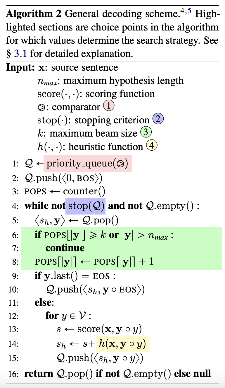
Best-First Beam Search: Core Insight

Paper: Best-first beam search (Meister et al., 2020)

Problem with Standard Beam Search:

Must analyze \(k\) hypotheses of given length before considering longer ones
Length-based prioritization is not necessary for finding \(k\)-optimal hypothesis
Computational inefficiency from rigid breadth-first expansion

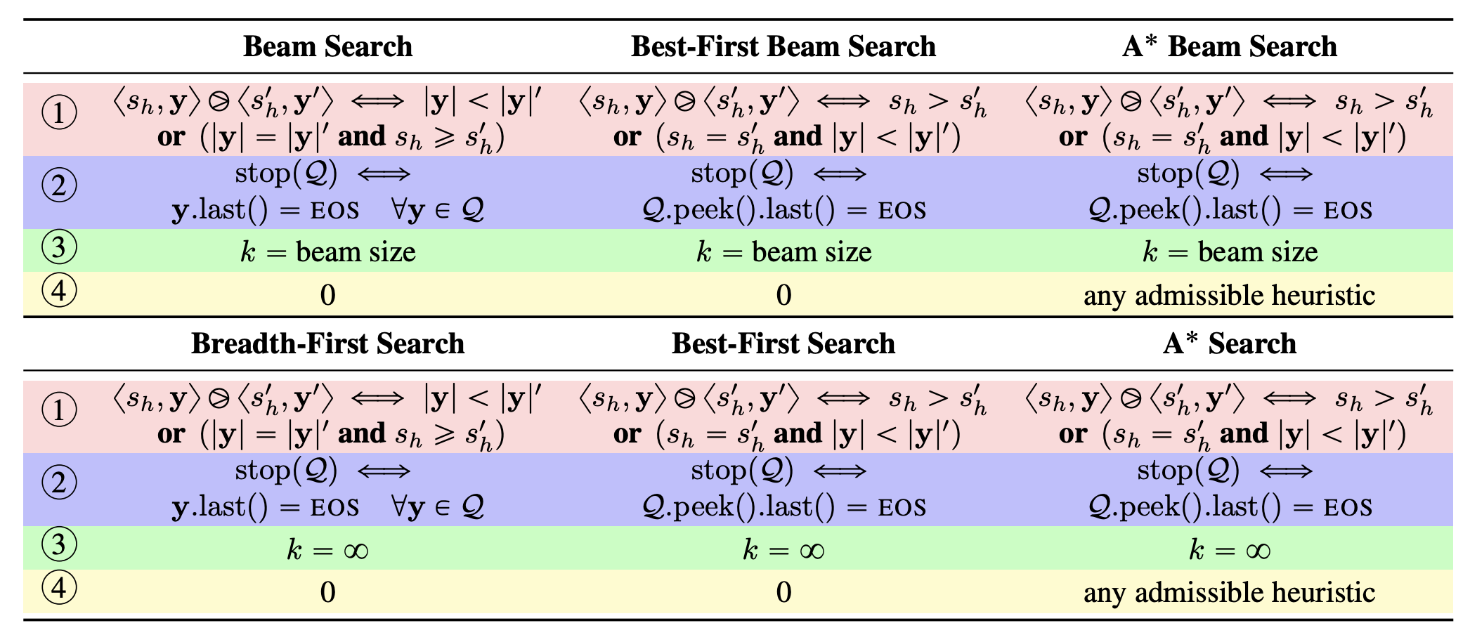
Key Insight: Use score-based prioritization like A* while maintaining beam constraints

Main Contribution: Up to 10x speedup over standard beam search with identical results

Best-First Beam Search: Algorithm

Key Insight: Use score-based prioritization like A* while maintaining beam constraints

Monotonicity Property: Scores can only decrease when extended

\[\text{score}(\mathbf{x}, \mathbf{y}_{\leq t}) \geq \text{score}(\mathbf{x}, \mathbf{y}_{\leq t} \circ y_{t+1})\]

Two Key Optimizations:

Early Pruning: Remove hypotheses guaranteed to fall off beam
Early Termination: Stop when first complete hypothesis found

Search Methods Comparison

Best-First Beam Search: Results

Performance Improvements:

2-10x speedup on neural machine translation
Identical BLEU scores to standard beam search
Greater speedups for larger beam sizes

When It Helps Most:

Large beam sizes (\(k \geq 10\))
Long sequences
High-quality models with good score separation

Trade-offs:

Memory overhead: \(O(k \cdot n_{\max})\) vs \(O(k)\)
Implementation complexity: More sophisticated data structures

A*esque Decoding Formulation

Paper: NeuroLogic Aesque Decoding: Constrained Text Generation with Lookahead Heuristics* (Lu et al., 2021)

States: Partial prefixes \(\mathbf{y}_{\leq t}\)
Actions: Tokens \(y_{t+1} \in \mathcal{V}\) (vocabulary)
Transitions: \(\mathbf{y}_{\leq t} \circ y_{t+1}\) (append token to prefix)

Objective: Find optimal sequence maximizing

\[\mathbf{y}_* = \arg \max_{\mathbf{y} \in \mathcal{Y}} f(\mathbf{y})\]

where \(f(\mathbf{y}) = s(\mathbf{y}) + h(\mathbf{y})\)

\(s(\mathbf{y}) = \log p_\theta(\mathbf{y})\) (log probability)
\(h(\mathbf{y})\) = constraint satisfaction score

A*-Inspired Lookahead Framework

Core Insight: Incorporate future estimates into candidate selection

Connection to Future Cost: Both use \(\text{score} = \text{current} + \lambda \cdot \text{heuristic}\)

Future Cost Approach

Heuristic: Learned predictor \(h(\mathbf{y}, \mathbf{x})\)
Training: Auxiliary loss to learn completion cost
Computation: Single forward pass
Generalization: Requires retraining for new domains

NeuroLogic A*esque Approach

Heuristic: Generated continuations \(h(\mathbf{y}_{\leq t+\ell})\)
Training: No additional training needed
Computation: Multiple forward passes for lookahead
Generalization: Works with any pre-trained model

A*esque Formulation:

\[Y_t = \arg \max_{k} \left\{s(\mathbf{y}_{\leq t}) + h(\mathbf{y}_{\leq t+\ell})\right\}\]

where \(h(\mathbf{y}_{\leq t+\ell}) = \lambda \log p_\theta(\mathbf{y}_{t+1:t+\ell}|\mathbf{y}_{\leq t}, \mathbf{x})\)

NeuroLogic A*esque: Constrained Generation

Key Innovation: Future constraint satisfaction estimation

Constraint Format: Include/exclude specific phrases

Example: Include “cat” and “fish” in generated text

Enhanced Scoring:

\[f(\mathbf{y}_{\leq t+\ell}) = \text{probability} + \text{current constraints} + \text{future constraints}\]

Future Constraint Heuristic: Estimate probability of satisfying constraints in lookahead continuations

Benefits: Early detection of constraint violations, better planning toward satisfiable paths

NeuroLogic A*esque: Algorithm & Results

Algorithm Steps:

Expand: Generate candidate continuations
Lookahead: For each candidate, generate length-\(\ell\) continuations
Score: \(f(\mathbf{y}_{\leq t+\ell}) = s(\mathbf{y}_{\leq t}) + h(\mathbf{y}_{t+1:t+\ell})\)
Select: Top-k candidates based on combined score
Prune: Remove constraint-violating candidates

Key Results:

+1.2-2.1 BLEU improvement over beam search
95%+ constraint satisfaction vs. 60-70% for baselines
Better coherence in long-form generation
Reduced myopia: Considers future implications vs. greedy decisions

Summary

Key Takeaways:

Classical search algorithms face challenges with transformer LMs
Approximate methods enable practical optimal search
Heuristic design is crucial for search quality
Best-first approaches often outperform standard beam search
Constraint satisfaction can be integrated into search

Next Class: Other controlled generation methods and their search implications